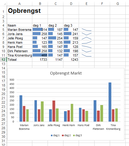


2. Cell properties
In this lesson you will learn how to format an Excel 2013 sheet and how to work with quick analysis.
Setting cell properties
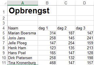
Recreate the table below:
Figure 2.1 Sponsored run
Make sure the Home tab is selected
Figure 2.2 Home tab
Select cells B5 to D11
Click the arrow  behind the menu
The Format Cells menu opens.
Figure 2.3 Format Cells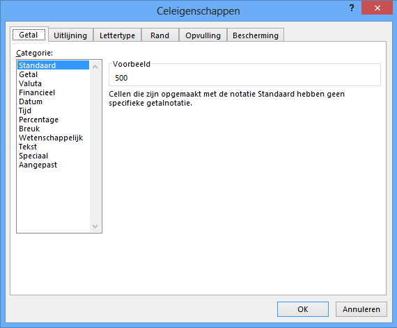
Select the Currency category
Figure 2.4 Cell properties currency
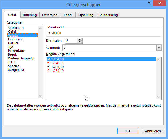
Make sure the euro symbol is selected and that the amount is displayed with 2 decimal places.
Type Total in A12
In B12, you enter a formula to calculate the total
Select cells B5 to B11
Figure 2.5 Selecting
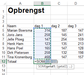
Click the SUM button
If you select cell B12 you can view the formula.
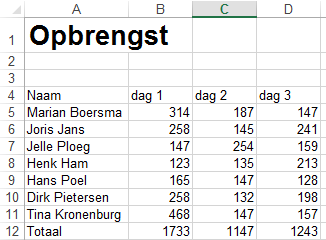
Calculate the totals for the other classes in the same way.
Figure 2.6 The totals in row 12
Quick Analysis
Select cells A4 to D11.Figure 2.7 Selecting
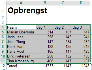
Figure 2.8 Right mouse button
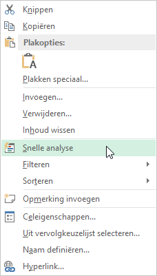
Figure 2.9 Quick Analysis
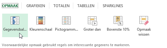
Select A4 to D11 again.
Figure 2.10 Selecting
Figure 2.11 Chart
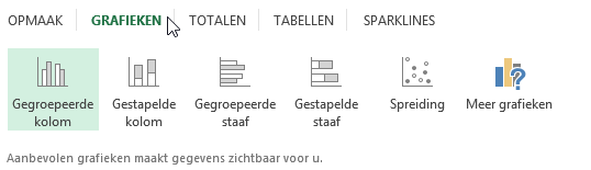
Figure 2.12 Resulting chart
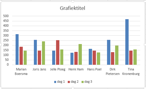
Quick Analysis gives you several ways to make data insightful.
Besides charts, you can also add Sparklines.
Make sure the data A4 to D11 is selected.
Again, use the right mouse button to choose Quick Analysis.
Now choose Sparklines; in this example, line has been selected.
Figure 2.13 Quick Analysis Sparkline
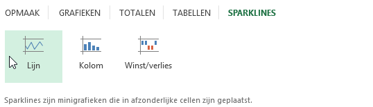
Figure 2.14 Result