1. Boodschappenlijst maken in Excel

We are going to make a list to keep track of the cost of the groceries.
Open Excel
You will see a blank sheet.

Type Groceries in A1
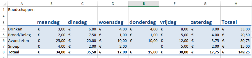
Turn the groceries table into a table, as shown in the example below.

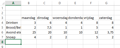
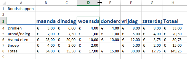
The text does not fit neatly into the columns, so we are going to make them wider.
The columns are indicated by letters.
First we will make column A wider.
Move your mouse over the column divider between column A and column B
The cursor changes into a double-headed arrow.

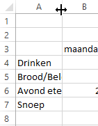
Drag the column border so that all the text fits in column A.
(you drag by holding down the left mouse button)

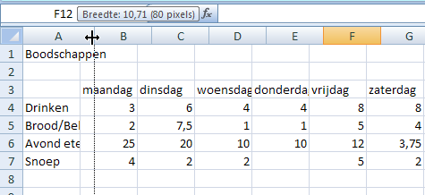
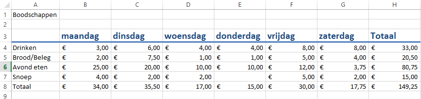
Make sure all columns are wide enough.

Calculating

The prices of the groceries have all been entered now. Next we are going to calculate how much was spent on groceries per day.

Type Total in cell A8
Go to cell B8
Type =B4+B5+B6+B7
Press Enter

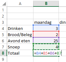
Calculate the total for Tuesday in the same way.

Calculating totals can also be done more quickly in Excel. This can be done using the SUM button.

Place the cursor in cell D8
Click the SUM button
Select cells D4 to D7
Press Enter

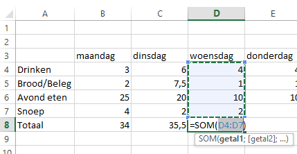
Now create the formula in E8 as well

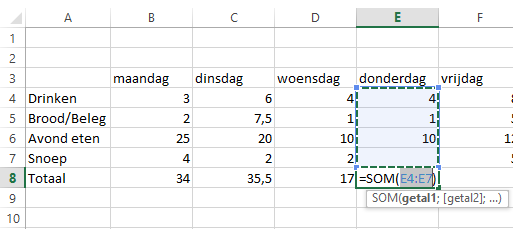
Also calculate the totals for Friday and Saturday.

Column H will contain the totals for a week.
Type Total in cell H3
Select cell H4
Click the Sum button
Check whether the correct cells are selected

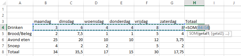
Press Enter

What formula has appeared in cell H4?

H4 now contains the correct formula.

We can drag these along using the fill handle.
Select cell H4
If you move your mouse over the bottom right-hand corner of the cell, the cursor changes into a black plus sign.

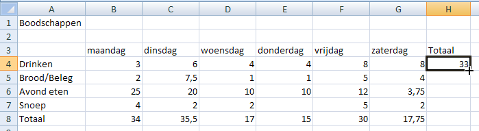
Hold down the left mouse button.
Drag down

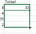
Excel also creates the formulas for the other cells.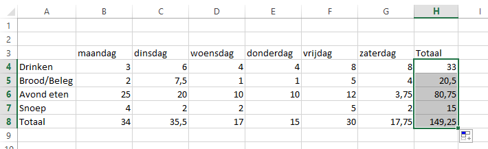

Look at the formulas.

Formatting

The calculations are complete, but it looks tidier to display the figures in euros.
Select the table

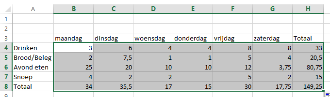
Once the numbers are selected, euro signs can be placed in front of them.
Click the currency button.

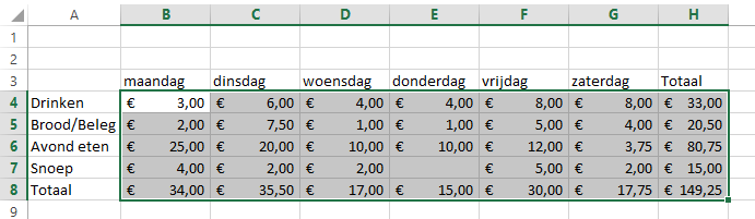
The numbers have been converted into euro amounts.

Cell styles

Now we are going to format the table with colours as well.

Select cells A3 to H3

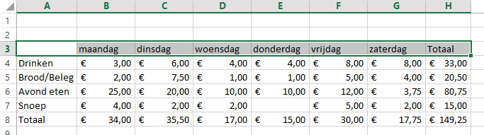
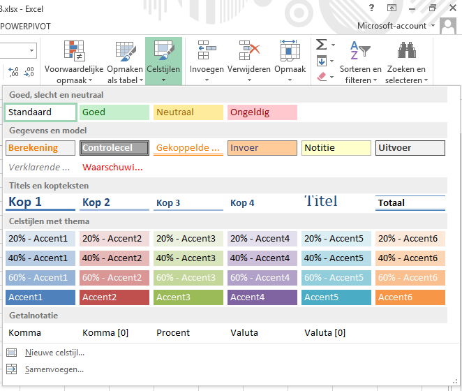
Click the Cell Styles button

Choose a format; in this example we use Heading 1

The formatting has been added to the table

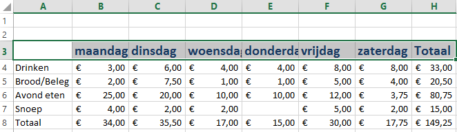
If the text no longer fits neatly in the cells, you can adjust this by making the columns wider.
Adjust the column width so that the text fits neatly within the cells.

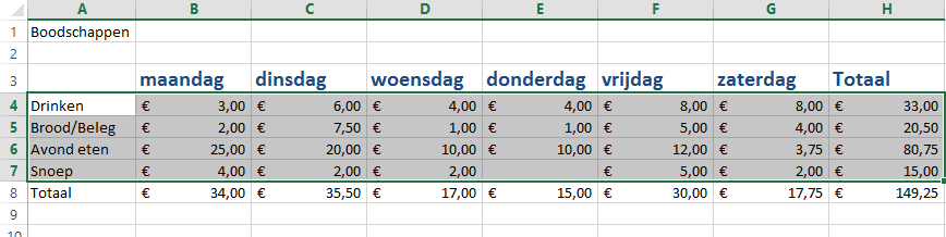
Select cells A4 to H7

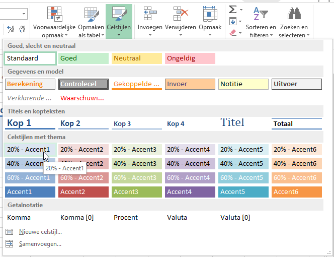
Click the Cell Styles button

Choose a format; in this example we use 20% Accent1

Finally, we add the formatting to the totals row.
Select cells A8 to H8
Click the Cell Styles button

In this example the format Total has been chosen

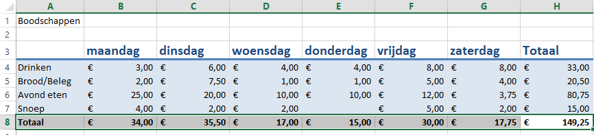
The result